
Introduction
Recently, a new neural network inspired by the Kolmogorov-Arnold theorem emerged—named the Kolmogorov Arnold Network (KAN). Proposed as an alternative to traditional Multi-Layer Perceptrons (MLPs), KAN aims to deliver strong predictive performance and excels particularly in interpretability, a key aspect of Explainable AI (XAI) [1].
What captivates me about KAN is how transparently it explains why certain predictions occur. This is especially valuable in finance, where understanding predictions can matter as much as accuracy itself.
In this blog post, I’ll walk through using KAN to predict stock prices and explore its interpretability advantages.
Fetching the Data
We fetched historical stock data for Apple (AAPL) using the yfinance library:
import yfinance as yf

start_training = '2021-01-01'
end_training = '2023-01-01'
start_testing = '2023-01-02'
end_testing = '2023-03-30'
ticker = "AAPL"

training_data = yf.download(ticker, start=start_training, end=end_training)
testing_data = yf.download(ticker, start=start_testing, end=end_testing)
Preparing the Data
We selected relevant features (Open, Low, High, Close) and scaled the data using MinMaxScaler:
from sklearn.preprocessing import MinMaxScaler
import numpy as np

features = ['Open', 'Low', 'High', 'Close']
scaler = MinMaxScaler()

train_scaled = scaler.fit_transform(training_data[features])
test_scaled = scaler.transform(testing_data[features])

def create_sequences(data):
    X, y = [], []
    for i in range(len(data)-1):
        X.append(data[i])
        y.append(data[i+1][3])  # Predict next day's Close price
    return np.array(X), np.array(y).reshape(-1,1)

X_train, y_train = create_sequences(train_scaled)
X_test, y_test = create_sequences(test_scaled)
Defining and Training the KAN Model
We defined and trained the KAN model:
from kan import KAN
import torch
import torch.nn as nn
import torch.optim as optim

kan = KAN(width=[4,8,4,1], grid=100, k=5, seed=42, device='cpu')

criterion = nn.MSELoss()
optimizer = optim.Adam(kan.parameters(), lr=0.002)

X_train_tensor = torch.tensor(X_train, dtype=torch.float32)
y_train_tensor = torch.tensor(y_train, dtype=torch.float32)

for epoch in range(100):
Evaluating the Model
We evaluated our model performance with unseen data:
from sklearn.metrics import mean_absolute_error, mean_squared_error

kan.eval()
X_test_tensor = torch.tensor(X_test, dtype=torch.float32)

with torch.no_grad():
    y_pred_scaled = kan(X_test_tensor).numpy().flatten()

combined_pred = np.hstack((X_test[:, :3], y_pred_scaled.reshape(-1, 1)))
combined_actual = np.hstack((X_test[:, :3], y_test))

y_pred_rescaled = scaler.inverse_transform(combined_pred)[:, 3]
y_actual_rescaled = scaler.inverse_transform(combined_actual)[:, 3]

mae = mean_absolute_error(y_actual_rescaled, y_pred_rescaled)
rmse = np.sqrt(mean_squared_error(y_actual_rescaled, y_pred_rescaled))

print(f"Mean Absolute Error (MAE): {mae:.4f}")
print(f"Root Mean Squared Error (RMSE): {rmse:.4f}")
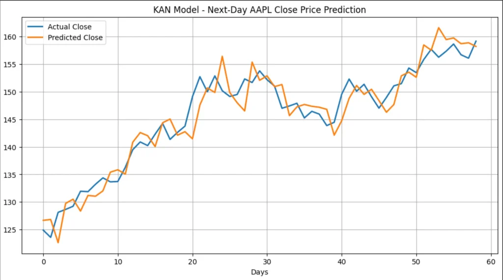
Our results were:
- Mean Absolute Error (MAE): 2.2516
- Root Mean Squared Error (RMSE): 2.7858
Predictions vs. actual prices visualization:
Why Use KAN Instead of an MLP?
KAN’s greatest advantage is interpretability. Unlike traditional “black box” neural networks, KAN clearly illustrates feature impacts via spline-based activations.
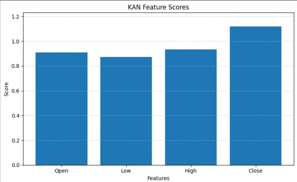
Global Feature Importance
We visualized global feature importance using pykan‘s built-in feature scoring function:
feature_scores = kan.feature_score.detach().cpu().numpy()This produced the following visualization clearly showing the relative importance of each feature:
Inspecting how the model adapts to training through analysing the Splines
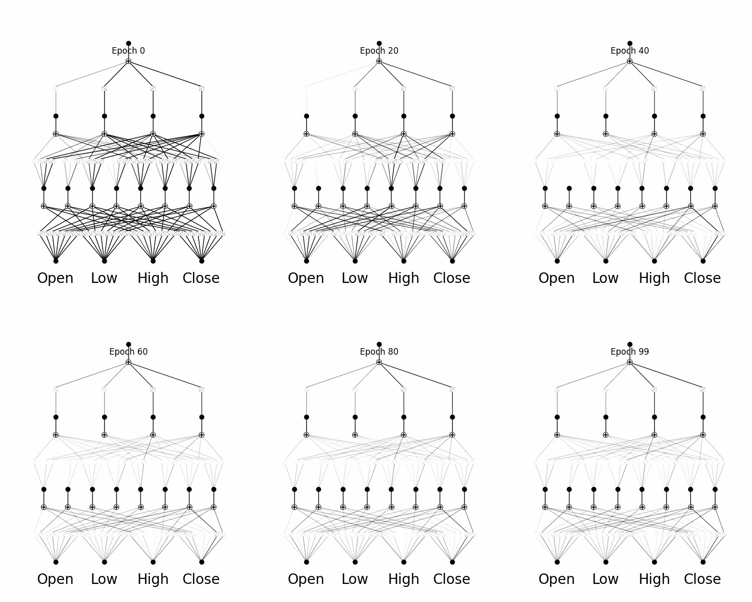
By utilising pykan’s ‘model.plot()’ function throughout training, we are able to see how the Kolmogorov Arnold Network’s B-splines adapt to the training data.
Inspecting Individual Splines
KAN allows inspection of individual spline functions, providing deeper insights into feature relationships. For example, we examined one specific spline from the model:
kan.get_fun(2,1,0)Here is an example spline visualization:
Inspecting splines helps understand exactly how inputs contribute to model outputs.
Conclusion
Kolmogorov Arnold Networks combine strong predictive performance with exceptional interpretability, making them particularly appealing in financial applications where transparency is crucial. This demonstration highlights the significant potential of KAN to provide explainable, trustworthy predictions. All code and theories outlined in this blog post are for educational purposes only and is not financial advice.
Recommended Resource
For additional insights and practical tips on KAN, I highly recommend visiting this excellent guide by Daniel Bethell. It’s been an incredibly helpful resource in my exploration.